- Information
- AI Chat
Excel Pretest - 123
Honors Exposition English (ENGLSH 1000H)
University of Missouri

Recommended for you


Preview text
ts ct?
1 Click the Name Box. 1/1 You clicked the Name
2 Apply the Accounting Number Format to the selected cells.
1/1 In the Home Ribbon Ta the Number Format d Format menu, youselec
3 Apply the Short Date format similar to 7/1/2016 to the selected cells.
1/1 In the Home Ribbon Ta the Number Format d Format menu, youselec
4 Apply the date number format to the selected cells to display dates in the format similar to 14-Mar.
1/1 In the Home Ribbon Ta Number Dialog Laun the Category list, you c Cells dialog from the Ty the Format Cells dialog
5 Use AutoFill to complete the series from cell B4 through cell D4.
1/1 You dragged the Fill H
6 Edit the formula in cell B9 so the references to cell E2 will update when the formula is copied, and the reference to cell B8 will remain constant. Use AutoFill to copy the formula to cells B10:B.
1/1 You clicked the formula cell C9 , clicked cell B typed " _=E2$B$8_* " in t Handle tool.
7 Use AutoSum to enter a SUM function in the selected cell.
1/1 In the Home Ribbon Ta the AutoSum button. Y
8 Create a new file based on the Personal expenses calculator template.
1/1 You opened the backst the Personal expense
9 Remove the fill color from the selected cells. 1/1 In the Home Ribbon Ta Color button arrow. In t
1 0
Apply the Calculation cell style to the selected cells. 1/1 In the Home Ribbon Ta Styles button. In the C
1 1
Use Format Painter to copy the formatting from cell E1 and apply it to cell F.
1/1 In the Home Ribbon Ta the Format Painter b
ts ct?
1
2
Apply conditional formatting to the selected cells using the blue solid fill data bar.
1/1 In the Home Ribbon Ta the Conditional Form the Data Bars menu, yo Gradient Blue option.
1 3
Apply conditional formatting to the selected cells using the Three Symbols (Circled) icon set (the first icon set in the Indicators section).
1/1 In the Home Ribbon Ta the Conditional Form the Icon Sets menu, yo Symbols Circled optio
1 4
Apply conditional formatting so cells with a value greater than the average are formatted using a yellow fill with dark yellow text.
1/1 Inside the Above Avera with drop-down. Inside range with drop-down, y Text list item. Inside th
1 5
Replace all instances of the word Spa Pool in this worksheet with Pool. Do not replace them one at a time. Close the dialog when you are finished.
1/1 Inside the Find and Rep Pool" , updated the Rep All button. Inside the M the Find and Replace d
1 6
Set the print area. 1/1 In the Page Layout Rib the Breaks button, clic Area menu, youclicked
1 7
Change the color of the sheet tab for the PO Q4 worksheet to Blue, Accent 1, Lighter 60% (the fifth option in the third row of theme colors).
1/1 You clicked the PO Q clicked the PO Q4 tab, the PO Q4 tab, right cl the Tab Right Click men Accent 1, Lighter 60%
1 8
Copy the Car Loan worksheet to a new workbook. 1/1 In the Tab Right Click m Inside the Move Or Cop clicked the To book dr book drop-down, you c Copy dialog, you clicke
1 9
Group together the Q1-Q2 and Q3-Q4 worksheets. 1/1 You shift-clicked the Q3-
ts ct?
Time menu, you clicked Arguments dialog, you
3 1
Insert the current date in the selected cell. Do not include the current time.
1/1 In the Formulas Ribbon the Date & Time butto the TODAY menu item. the OK button.
3 2
In cell C12, enter a formula using a counting function to count the number of items in the Item column (cells C2:C11 ).
1/1 You typed =Counta(C2:C11)
3
3
In cell G12, enter a formula using a counting function to count the number of blank cells in the Received column (cells G2:G11 ).
1/1 You typed =COUNTBLA
3
4
In cell F12, enter a formula using a counting function to count numbers in the Ordered column (cells F2:F11 ).
1/1 You typed =COUNT(f2:f
3
5
Enter a formula in cell B8 to display the text from cell A8 in all lower case letters.
1/1 You typed =LOWER(A8)
3
6
Enter a formula in cell B8 to display the text from cell A8 in proper case with only the first letter of each word in upper case.
1/1 You typed =Proper in
3
7
Enter a formula in cell B8 to display the text from cell A8 in all upper case letters.
1/1 You typed =uppe in ce
3
8
On the Summary sheet, in cell B3, enter a formula to display the value of cell B3 from the ByMonth sheet.
1/1 You typed = in cell B3 , and clicked cell B.
3 9
Name cell B1 as follows: BonusRate 1/1 In the Formulas Ribbon the Define Name butt the Define Name... m the OK button.
4 0
Use the Create from Selection command to create named ranges for the data table B8:E11 using the
1/1 In the Formulas Ribbon the Create from Sele
ts ct?
labels in row 1 as the basis for the names. Selection dialog, you c
4 1
Enter a formula in cell B2 to calculate Ken Dishner's bonus for the first quarter. Multiply his sales total (cell E8 ) times the bonus rate (the cell named BonusRate ).
1/1 You typed =E8*Bo in c pressed Enter.
4
2
Edit the Bonuses named range so it refers to cells B2:B5 on the Bonus worksheet. Close the Name Manager when you are finished.
1/1 In the Formulas Ribbon the Name Manager b the close dialog butto Refers Input , clicked th
4 3
Enter a formula in cell C2 to return a value of yes if the value in cell E8 is greater than or equal to the value in B2 or no if it is not.
1/1 In the Logical menu, yo Arguments dialog, you the If Logical Test Form Input , typed "no" in th Value If False Formu
4 4
Using cell references , enter a formula in cell B7 to calculate monthly payments for the loan described in this worksheet. Use a negative value for the Pv argument.
1/1 In the Financial menu, Arguments dialog, you the Pmt Rate Formula In typed -B4 in the Pmt P
4 5
Enter a formula in cell B2 using the VLOOKUP function to find the total sales for the date in cell B1. Use the name DailySales for the lookup table. The total sales are located in column 5 of the lookup table. Be sure to require an exact match.
1/1 Inside the Function Arg typed False in the Vloo the Vlookup Lookup Va Table Array Formula Inp Input , and clicked the O
4 6
Show the tracer arrows from cell B5 to the cell(s) that are dependent on it (cells containing formulas that reference the value or formula in cell B5).
1/1 In the Formulas Ribbon Group, you clicked the
4
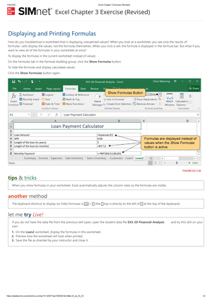
7
Display the formulas in this worksheet. 1/1 In the Formulas Ribbon Group, you clicked the
4 8
Enter a formula in cell D2 to calculate C2/C14 rounded to 3 decimal places.
1/1 You typed =Round(C2/
ts ct?
typed ">14" in the Cou
5 5
In cell H2, enter a formula using COUNTIFS to count the number of rows where values in the range named Delivery Time have a value greater than 14 and cells in the range named ReorderStatus display "no".
1/1 Inside the Function Arg typed Delivery Time i typed ">14" in the Cou typed ReorderStatus typed "no" in the Coun the OK button.
5 6
Enter a formula in cell E2 to calculate the median value of the prices in the cell range C6:C.
1/1 You typed =MEDIAN(C6:C14)
5
7
Enter a formula in cell C1 to calculate the standard deviation of the values in cells C5:C13. Assume this array is a sample of a larger set of values.
1/1 In the More Functions m S menu item. Inside the dialog button, typed C5:C keydowned the Stdev.
5 8
Enter a formula in cell C1 to find the rank of the value in cell C9 compared to the values in cells C5:C.
1/1 In the More Functions m Eq menu item. Inside th dialog button, typed C typed C5:C13 in the Ra the Rank Ref Form
5 9
In cell D6, enter a formula using OR to display TRUE if the daily sales (cell C6 ) is greater than the overall average (cell C3 ) or the daily sales (cell C6 ) is greater than the employee's average (cell C4 ). Use cell references and enter the arguments exactly as described in this question.
1/1 In the Logical menu, yo Arguments dialog, you the Or Logical1 Formul Input , and keydowned
6
0
In cell D6, enter a formula using AND to display TRUE if the daily sales (cell C6 ) is greater than the overall average (cell C3 ) and the daily sales (cell C6 ) is greater than the employee's average (cell C4 ). Use cell references and enter the arguments exactly as described in this question.
1/1 In the Logical menu, yo Arguments dialog, you the And Logical1 Formu Input , and keydowned
6
1
In cell B6, enter a formula to calculate the future value of this savings strategy. Use cell references wherever
1/1 In the Financial menu, Arguments dialog, you
ts ct?
possible. The annual interest rate is stored in cell B5 , the number of payments in cell B4 , and the monthly payment amount in cell B3. Remember to divide the annual interest rate by 12 and use a negative value for the Pmt argument.
the Fv Rate Formula In B3 in the Fv Pmt Formu Input collapsible input
6
2
In cell B10, enter a formula using PV to calculate the value today (the present value) of the four-year tuition plan. Use cell references wherever possible. The annual interest rate for your investment account is stored in cell B8 , the number of monthly payments in cell B7 , and the monthly payment amount in cell B. Payments will be made at the beginning of every period. Pay attention to the time periods for the interest rate and payment schedule. Remember to express the Pmt argument as a negative.
1/1 In the Financial menu, Arguments dialog, you the Pv Rate Formula In b6 in the Pv Pmt Formu clicked the OK button.
6
3
In cell B14, enter a formula using NPV to calculate the value today (the present value) of the tuition payment option 3. Use cell B7 as the Rate argument and the cell range B10:B13 as the Value1 argument. Use cell references for all values.
1/1 In the Financial menu, Arguments dialog, you Rate Formula Input , typ keydowned the Npv Va
6
4
In cell B8 , enter a formula using NPER to calculate how many payments are left on this student loan. The annual interest rate is in cell B4. The monthly payment is in cell B7. The current value of the account is in cell B2. Payments will be made at the beginning of every period. Remember to adjust the interest rate to reflect the same time period as the payments and to express the Pmt argument as a negative.
1/1 In the Financial menu, Arguments dialog, you the Nper Rate Formula typed b2 in the Nper Pv Input , and keydowned
6
5
In cell B5, enter a formula using the function for the Declining balance depreciation method. Use the cell names Purchase , Sale , and Life for the function arguments. Use a relative reference to cell A5 for the Per argument. Enter a partial year of 4 months in the Month argument.
1/1 Inside the Function Arg typed Purchase in the Number2 Formula Inpu typed a5 in the Db Num Formula Input , and clic
Excel Pretest - 123
Course: Honors Exposition English (ENGLSH 1000H)
University: University of Missouri


- Discover more from: