
- Information
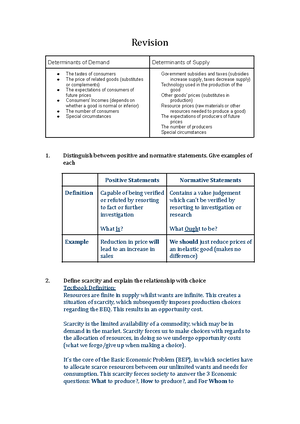
- AI Chat
Mathematical investigation of an egg - Grade: A
Mathematics: Analysis and Approaches SL
IB
High School - US
Recommended for you


Related documents
- Math skill Half-life and KEY
- IA Mathematics SL - IB diploma may 2019
- Math IA Finding the Shortest Cycle in the Neighborhood
- Doraemon- Grade: A
- Mathematics Investigation: How many ways can a number of telephones be connected if a telephone can't connect to more than one other? - Grade: A
- Public-Key Cryptography - Grade: A
Related Studylists
Daniel C J Mishael studyPreview text
MATHEMATICS IA
Mathematical investigation of an egg
Date of submission: March 2020 Exam Session: May 2020 Submitted by: hxp
1. INTRODUCTION
Using knowledge and theories from the sciences and applying it to real-life situations in order to help with problem solving has always been intriguing to me; this is an important aspect of being an inquirer, one of the IB learner profile traits. For example, in HL Chemistry, we carried out a lab experiment involving titrations in order to calculate the mass of calcium carbonate present in a sample of eggshell. I was able to use my existing knowledge of reactions and mole calculations in order to acquire new information which is of potential significance to the industry; studies have suggested that calcium carbonate extracted from eggshell is a good pharmaceutical excipient that can be used in a variety of products (Murakami et al., 2007). Similarly, I wanted to employ my mathematical knowledge to do something which I found interesting and provides useful information in contextual real-life situations.
As a child, when I was living in Egypt, I remember helping my grandmother in taking care of the farm animals. She would always ask me to go count how many eggs the chicken have laid and bring some to her. While doing so, I would observe the eggs and ponder over their elegant shape, and then talk about it with her. I was fascinated by how myriad complex shapes were present in nature, sparking an interest within me. As I developed a passion for mathematics, I started thinking about such phenomena from a mathematical point of view, and so I decided to model a chicken egg in this exploration, viewing the problem from different perspectives and using different approaches. This investigation aims to find suitable mathematical models for a chicken egg and comparing them, and further, to calculate the volume and surface area of the egg from those models. This topic is relevant and has wider implications; the volume is indicative of the amount of yolk in the egg, while the surface area is indicative of the amount of eggshell present. The egg I modelled was randomly taken from the kitchen and is shown in Figure 1.
2 Method A: Modifying the Ellipse Equation The shape of an egg is somewhat similar to that of an ellipse, therefore it could be used as a good starting point. An ellipse has two different “radii”, defined as the major axis and the minor axis. The equation of a general ellipse is as follows: ݔଶ ݎ௫ଶ+
ݕଶ
ݎ௬ଶ= ͳ , ሺͳሻ
where ݎ±௫ and ݎ±௬ represent the ݔ and ݕ axes-intercepts respectively. They could also be thought of as the horizontal and vertical radii. The one with the greater magnitude represents the major axis, while the other is the minor axis. The magnitude of either of the axes is simply twice the value of ݎ௫ or ݎ௬, i. the distance between the two vertical or horizontal intercepts. In
order to simplify upcoming calculations, the denominators in (1) will be replaced with ܽ and ܾ, as follows: ݔଶ ܽ +
ݕଶ
ܾ = ͳ ሺʹሻ By composing (2) with a function, either in terms of ݔ or ݕ, the ellipse could be modified to further resemble the shape of an egg. This function could take any form, but let us consider the simple, judicious case in which we add a term ‘ݕܿ’ to the denominator: ݔଶ ܽ +
ݕଶ
ݕܿ + ܾ= ͳ,where c > Ͳ ሺ͵ሻ Here, ܿ is another parameter which—in colloquial terms—‘controls’ the shape of the ellipse above and below the ݔ-axis, such that it stops looking like an ellipse and more like an egg. Figure 3 highlights this difference and shows how (3) resembles an egg much better than (2) does. We can understand why this works by considering the symmetry of the ellipse. The denominator is a constant value, ܾ, giving the same vertical radius above and below the ݔ-axis; however, upon adding another term to the denominator which is dependent on ݕ, the symmetry changes, altering the shape. Below the ݔ-axis, since the ݕ values are negative, the magnitude
of the term ‘ݕܿ + ܾ’ would decrease (when ܿ is positive). In contrast, the magnitude would increase above the ݔ-axis because the ݕ values are positive. As such, this asymmetry results in different distances from the origin for different points on the curve. The larger the value of ܿ, the more drastic this asymmetry is above and below the ݔ-axis. Negative values of ܿ would simply rotate the curve by ͳ ͅͲ°, and therefore the restriction on ܿ was applied since the egg being modelled in Figure 2 contains the “smaller radius” below the ݔ-axis.
Now, we can try applying this general model to our egg, in which case we will need to find appropriate values for our three parameters ܽ, ܾ and ܿ. In order to do this, a system of at least three linear equations will be needed, and hence at least three co-ordinates. The axes intercepts can be used as co-ordinates as that would simplify the calculation process, as these co-ordinates will help eliminate the ݔ or ݕ part of the equation. Looking back at Figure 2, we can see that the egg intercepts the ݕ-axis at (0, 3) and (0, –2), and the ݔ-axis at (±ʹ.ͳ,Ͳሻ. Substituting these values into (3) yields the following system of equations: + ܾ͵.ʹ = ܿ͵.ʹଶ ሺͶሻ ܾ− ʹ.ʹ = ܿʹ.ʹଶ ሺͷሻ ʹ.ͳଶ ܽ = ͳ ሺሻ We can subtract (5) from (4) to give us:
Figure 3: Graphical representation of (3) in blue, and (2) in red.
doing, although that is not vital, since the current function is a decent representation that only minimally strays away from the ‘perfect’ shape.
2 Method B: Using Polynomials Note that in this section, to help with modelling, the egg in Figure 2 will be rotated ͻͲ° clockwise such that it is placed horizontally along the ݔ-axis. This method involves analytically finding polynomial equations that can model one half of the egg, and then reflecting them in the ݔ-axis to obtain the equations for the other half, assuming that the egg is symmetrical on both sides. These polynomial functions can be found using the Lagrange interpolation formula, which states that for a unique polynomial of degree ݊, ሺ݊ + ͳሻ data points are required to find a ‘best’ fit. The formula is given as follows for a polynomial ሻݔሺܲ:
ܲሺݔሻ = ∑ݔሺݔ − ݔሺ𥠀ݔ −ଵଵሻ.. .ሺݔሻ... ሺ ݔ− ݔ𥠀ݔ −𥠀−ଵ𥠀−ଵሻሺ ݔ− ݔݔሻሺ𥠀ݔ −𥠀+ଵ𥠀+ଵሻ. .. ሺ ݔ− ݔሻ.. .ሺݔ𥠀ݔ −+ଵ+ଵሻሻݕ𥠀
+ଵ 𥠀=ଵ where ͳ 𥠀 + ݊ͳ ݀݊ܽ ܲሺݔ𥠀ሻ = ݕ𥠀 (Brilliant, 2019) Needless to say, the higher the degree of the polynomial chosen, the more accurately the egg can be modelled. However, some preliminary testing showed that only one second, third, or fourth degree polynomial is not a decent fit for the egg (top half) in its entirety. This makes sense as the curvature of the egg is different from that of the nature of a quadratic or cubic or a quartic. We could, of course, try using higher degrees such as fifth or sixth degrees, although that would result in complicated polynomials that are unnecessarily long and would be time consuming to expand and simplify. As such, it could be helpful to divide the egg into three sections: left, middle and right, where each section can be modelled using a separate polynomial. I have chosen to simply use quadratic equations; in which case I will need three data points for each section. The Lagrange interpolation formula for a quadratic ( = ݊ʹ,𥠀 = ͵ሻ is then written as:
ܳሺݔሻ=ሺሺݔݔ − ݔଵݔ −ଶଶሻሺሻሺݔ − ݔݔଵݔ −ଷଷሻሻݕଵ+ሺݔሺݔ − ݔଶݔ −ଵଵሻሺሻሺݔ − ݔݔଶݔ −ଷଷሻሻݕଶ+ሺሺݔݔ − ݔଷݔ −ଵଵሻሺሻሺݔ − ݔݔଷݔ −ଶଶሻሻݕଷ ሺ ͅሻ
Using three randomly chosen co-ordinates from the ‘left’ section of the egg (given in Table 1), we can therefore find the quadratic equation, ܳሻݔሺ, to be:
ܳሺݔሻ =ሺ ݔ− Ͳ.ሺͲ − Ͳ.ʹͷ ሻሺ ݔ− Ͳ.ʹͷ ሻሺͲ − Ͳ.ͷͳʹ ሻͷͳʹ ሻሺͲ. Ͳͳ ሻ +ሺͲ. ʹͷ ሻሺͲ. ʹͷ − Ͳ. ͷͳʹ ሻݔሺ ݔ− Ͳ.ͷͳʹ ሻ ሺͲ. ͅ ͅ ሻ +ሺͲ. ͷͳʹ ሻሺͲ. ͷͳʹ − Ͳ. ʹͷ ሻݔሺ ݔ− Ͳ.ʹͷ ሻ ሺͳ. ʹ ͅ͵ ሻ ≈ −͵. ͅ ͅͶʹͶͶݔଶ+ Ͷ. ͶͷͲͳ + ݔͲ.Ͳͳ ሺ ݀. 𧐀. ሻ Note that the equation above was not simplified by expanding the linear expressions and summing them, as that would have been tedious and time consuming; rather, I inputted (8) into WolframAlpha to simplify the equation to a quadratic in the form ݔܽଶܿ + ݔܾ +, where:
= ܽݔሺଵݔ −ଶݕݔሻሺଵ ଵݔ −ଷሻ+ݔሺଶݔ −ଵݕݔሻሺଶ ଶݔ −ଷሻ+ݔሺଷݔ −ଵݕݔሻሺଷ ଷݔ −ଶሻ ܾ = −ݔሺଵݔ −ݔଶݔሻሺଷݕଵଵݔ −ଷሻ−ݔሺଵݔ −ݔଶݔሻሺଶݕଵଵݔ −ଷሻ−ݔሺଶݔ −ݔଵଷݔሻሺݕଶଶݔ −ଷሻ −ݔሺଶݔ −ݔଵݔሻሺଵݕଶଶݔ −ଷሻ−ݔሺଷݔ −ݔଵଶݔሻሺݕଷଷݔ −ଶሻ−ݔሺଷݔ −ݔଵଵݔሻሺݕଷଷݔ −ଶሻ = ܿݔሺଵݔ−ݔଶଶݔݔሻሺଷݕଵଵݔ−ଷሻ+ݔሺଶݔ−ݔଵଵݔݔሻሺଷݕଶଶݔ−ଷሻ+ݔሺଷݔ−ݔଶଵݔݔሻሺଷݕଷଵݔ−ଶሻ
I then simply inputted the expressions above and the co-ordinates’ values from the tables to calculate the quadratic coefficients using Desmos.
one output for each input. Looking at Figure 6, the piecewise relation seems to be an almost excellent model for the egg as it nearly overlaps with the outline of the egg perfectly; although the curvature seems to be one aspect which is lacking as the transitions between the quadratic functions at the different sections seem to be ‘awkward’ rather than smooth, i. it can easily be deduced that (9) is a piecewise relation solely from looking at the graph. Furthermore, the assumption that the egg is symmetrical about the x -axis seems to be true through observing the graph below and above the ݔ-axis, although it cannot be asserted that the egg is perfectly symmetrical. In order to achieve better accuracy, the Lagrange interpolation formula could have been applied for the bottom half too, but that would be unnecessary and time consuming merely for a minute increase in the level of accuracy.
Reflecting upon this method, it might have seemed somewhat unnecessary using the Lagrange interpolation formula to merely find the coefficients of quadratic equations. Perhaps, it could have been more efficient to construct three simultaneous equations with the unknown
Figure 6: Graphical representation of the piecewise relation (9).
coefficients ܽ, ܾ, and ܿ, and then perform Gaussian elimination to find their values, which would have resulted in the same values obtained from the Lagrange formula. Originally, this formula was introduced with the aim of finding one higher -order polynomial that would model the whole egg (which would have been difficult to do using other methods); however, the inability to do so alluded to dividing the egg into three quadratic sections, in which case the Lagrange formula would have not been necessary to do so. Although this method is unique and accurate, other methods could have been used to simplify the calculation process.
2 Comparing the Methods Perhaps the most notable difference between the two methods is that method A is more general than method B, as it can be easily applied to any unique egg possessing the same general shape, given the axes-intercepts of the egg. Method B on the other hand is more specific in the sense that many separate, different polynomial functions will be needed to model the egg. Although the second model seems to be a more accurate fit than the first (through comparing Figure 4 with Figure 6), the first model could be considered superior due to its higher generalizability; not to mention that its graph is continuous and appears to be smoother. As such, the model obtained from the first method, (7), will be used in upcoming calculations for the volume and surface area. That being said, each model is unique and has its own pros and cons.
3. CALCULATING THE VOLUME In HL math, we learnt that the volume of the solid generated by revolving a 2D function, ሻݕሺ݂, rotated 2 degrees about the ݕ-axis is given by evaluating the following integral between two desired limits:
∫[݂ሺݕሻ]ଶݕ݀
, ሺͳͲሻ
4. CALCULATING THE SURFACE AREA
As with the volume, it is possible to calculate the surface area of the solid generated by rotating the function ሻݕሺ݂ about the ݕ-axis, according to the following formula:
𝀀 = ʹ ∫ ݂ሺݕሻ√ͳ +[݂′ሺݕሻ]ଶݕ݀
ሺͳͶሻ (Weisstein, 2019) Solving for the positive solution of ݔ in (11):
= ݔʹ.ͳ√ͳ −. ͲͶ + ݕݕଶ ሺͳͷሻ
We can therefore compute the derivative ௗ௫ௗ௬ by using the chain rule for the square root function
followed by using the quotient rule for the term . ସ +௬௬ 2 :
ݔ݀ ݕ݀= ʹ.ͳ × Ͳ.ͷ (
ͳ √ͳ −. ͲͶ + ݕݕଶ )
ቆ−ݕʹሺሺ. ͲͶ + ݕ. ͲͶ + ݕሻሻݕ −ଶ ଶቇ
= −ͳ. Ͳͷሺݕ ଶ+ ͳͶ .Ͳ ͅ ݕሻ ሺ. ͲͶ + ݕሻଶ√ͳ −. ͲͶ + ݕݕଶ
ሺͳሻ
We can now use (14) to find the formula for the surface area, where ሻݕሺ݂ is given by (15), and ሻݕ′ሺ݂ is given by (16):
𝀀 = Ͷ.ʹ ∫√ͳ −. ͲͶ + ݕݕଶ ⋅√ͳ + (
−ͳ. Ͳͷሺݕଶ+ ͳͶ .Ͳ ͅ ݕሻ ሺ. ͲͶ + ݕሻଶ√ͳ −. ͲͶ + ݕݕଶ )
ଶ ݕ݀
ଷ.ଶ −ଶ.ଶ
A GDC was used to find the value of this integral, giving: 𝀀 = Ͷ.ʹ × ͷ.ͲͳͶ ͅͻͳʹ ≈ .ʹ ݉ܿଶ ሺ͵ ݂ .ݏ. ሻ
5. DISCUSSION
Since these calculated values of volume and surface area are likely to be overestimates (because the calculations were based on the model from Figure 4, which contained minor flaws as aforementioned), it may be worth finding a method to validate these values. This would also help in ensuring that the mathematics was correct. Conducting a displacement test would not have been a good solution as that would only provide a value for the volume, not to mention that it lacks precision. Upon researching, I found a seemingly highly accurate model by Nobuo Yamamoto (2007) which has a rigorous proof beyond the scope of this paper, as follows: ሺݔଶݕ +ଶሻଶݔܽ =ଷ+ሺܾ − ܽሻݕݔଶ, ሺͳሻ Ͳ ܾ ܽ ݁ݎ݁ ℎݓ ܽ and ܾ being parameters which change the shape of the egg curve. Using Desmos, I found their values which best fit my egg, as shown in the figure below:
It can be seen that the equation is a very accurate model of the egg and therefore we can be certain in the values obtained from the calculations. According to Yamamoto, the volume of revolution using this model can be calculated as:
ሺݔଶݕ +ଶሻଶ= ͷ. ͵͵ ݔଷ+ ʹ. ʹ ݕݔଶ
Figure 7: Nobuo Yamamoto equation for my egg; = ܽͷ.͵͵, = ܾʹ.ͳ
when measuring the length of the egg, which could have altered the values obtained from the calculations. For further investigations, it could be intriguing to use a number of different eggs and model them to determine a more generic and accurate model. Additionally, it could be worth investigating if there is a mathematical relationship between the length of an egg and its volume and/or surface area, possibly leading to some interesting mathematics involving statistical analyses of correlation coefficients.
REFERENCES
Brilliant (2019). Lagrange Interpolation. Available at: brilliant/wiki/lagrange- interpolation/ (Accessed: 5 December 2019)
Desmos Graphing Calculator. (n.). Desmos Graphing Calculator. Available at: desmos/calculator (Accessed: 1 December 2019)
Murakami, F., Rodrigues, P., Campos, C.M., Silva, M.A. (2007). Physiochemical study of CaCO 3 from eggshells. SciELO Analytics. dx.doi/10.1590/S
Weisstein, E. (2019). Surface of Revolution. From MathWorld --A Wolfram Web Resource. Available at: mathworld.wolfram/SurfaceofRevolution.html (Accessed: 7 December 2019)
WolframAlpha. (n.) Available at: wolframalpha (Accessed: 6 December 2019)
Yamamoto, N. (2007 ). Equation of Egg Shaped Curve of the Actual Egg is Found. Available at: nyjp07/index_egg_E.html (Accessed 8 December 2019)
Mathematical investigation of an egg - Grade: A
Subject: Mathematics: Analysis and Approaches SL
IB


- Discover more from:


Recommended for you
Students also viewed
Related documents
- Math skill Half-life and KEY
- IA Mathematics SL - IB diploma may 2019
- Math IA Finding the Shortest Cycle in the Neighborhood
- Doraemon- Grade: A
- Mathematics Investigation: How many ways can a number of telephones be connected if a telephone can't connect to more than one other? - Grade: A
- Public-Key Cryptography - Grade: A