
- Information
- AI Chat
Exam, answers
Data Mining (IS ZC425)
Recommended for you


Comments
- thanks
- Thank you
- Can't open it please help in opening


Related Studylists
ABDUL RAZACPreview text
SOLVED PAPERS
OF
DATA WAREHOUSING &
DATA MINING
(DEC-2013 JUNE- 2014 DEC- 2014 &
JUNE-2015)
A-
1b. What is ETL? Explain the steps in ETL. (07 Marks) Ans: ETL (EXTRACTION, TRANSFORMATION & LOADING)
- The ETL process consists of → data-extraction from source systems → data-transformation which includes data-cleaning & → data-loading in the ODS or the data-warehouse.
- Data cleaning deals with detecting & removing errors/inconsistencies from the data.
- Most often, the data is sourced from a variety of systems.
PROBLEMS TO BE SOLVED FOR BUILDING INTEGRATED-DATABASE
- Instance Identity Problem
- The same customer may be represented slightly differently in different source- systems.
- Data-errors
- Different types of data-errors include: i) There may be some missing attribute-values. ii) There may be duplicate records.
- Record Linkage Problem
- This deals with problem of linking information from different databases that relates to the same customer.
- Semantic Integration Problem
- This deals with integration of information found in heterogeneous-OLTP & legacy sources.
- For example, → Some of the sources may be relational. → Some sources may be in text documents. → Some data may be character strings or integers.
- Data Integrity Problem
- This deals with issues like i) referential integrity ii) null values & iii) domain of values. STEPS IN DATA CLEANING
- Parsing
- This involves → identifying various components of the source-files and → establishing the relationships b/w i) components of source-files & ii) fields in the target-files.
- For ex: identifying the various components of a person„s name and address.
- Correcting
- Correcting the identified-components is based on sophisticated techniques using mathematical algorithms.
- Correcting may involve use of other related information that may be available in the company.
- Standardizing
- Business rules of the company are used to transform data to standard form.
- For ex, there might be rules on how name and address are to be represented.
- Matching
- Much of the data extracted from a number of source-systems is likely to be related. Such data needs to be matched.
- Consolidating
- All corrected, standardized and matched data can now be consolidated to build a single version of the company-data.
- Instance Identity Problem
A-
1c. What are the guide lines for implementing the data-warehouse. (05 Marks) Ans: DW IMPLEMENTATION GUIDELINES Build Incrementally - Firstly, a data-mart will be built. - Then, a number of other sections of the company will be built. - Then, the company data-warehouse will be implemented in an iterative manner. - Finally, all data-marts extract information from the data-warehouse. Need a Champion - The project must have a champion who is willing to carry out considerable research into following: i) Expected-costs & ii ) Benefits of project. - The projects require inputs from many departments in the company. - Therefore, the projects must be driven by someone who is capable of interacting with people in the company. Senior Management Support - The project calls for a sustained commitment from senior-management due to i) The resource intensive nature of the projects. ii ) The time the projects can take to implement. Ensure Quality - Data-warehouse should be loaded with i) Only cleaned data & ii) Only quality data. Corporate Strategy - The project must fit with i) corporate-strategy & ii) business-objectives. Business Plan - All stakeholders must have clear understanding of i) Project plan ii) Financial costs & iii) Expected benefits. Training - The users must be trained to i) Use the data-warehouse & ii) Understand capabilities of data-warehouse. Adaptability - Project should have build-in adaptability, so that changes may be made to DW as & when required. Joint Management - The project must be managed by both i) IT professionals of software company & ii) Business professionals of the company.
2a. Distinguish between OLTP and OLAP. (04 Marks) Ans:
A-
PIVOT (OR ROTATE)
- This is used when the user wishes to re-orient the view of the data-cube. (Figure 2).
- This may involve → swapping the rows and columns or → moving one of the row-dimensions into the column-dimension.
Figure 2: Pivot operation SLICE & DICE
- These are operations for browsing the data in the cube.
- These operations allow ability to look at information from different viewpoints.
- A slice is a subset of cube corresponding to a single value for 1 or more members of dimensions. (Figure 2).
- A dice operation is done by performing a selection of 2 or more dimensions. (Figure 2).
Figure 2: Slice operation Figure 2: Dice operation
A-
2c. Write short note on (08 Marks) i) ROLAP ii) MOLAP iii) FASMI iv) DATACUBE Ans:(i) For answer, refer Solved Paper June-2014 Q.No. Ans:(ii) For answer, refer Solved Paper June-2014 Q.No. Ans:(iii) For answer, refer Solved Paper June- 201 5 Q.No. Ans:(iv) For answer, refer Solved Paper Dec-2014 Q.No.
3a. Discuss the tasks of data-mining with suitable examples. (10 Marks) Ans: DATA-MINING
- Data-mining is the process of automatically discovering useful information in large data- repositories. DATA-MINING TASKS
- Predictive Modeling
- This refers to the task of building a model for the target-variable as a function of the explanatory-variable.
- The goal is to learn a model that minimizes the error between i) Predicted values of target-variable and ii) True values of target-variable (Figure 3).
- There are 2 types: i) Classification: is used for discrete target-variables Ex: Web user will make purchase at an online bookstore is a classification-task. ii) Regression: is used for continuous target-variables. Ex: forecasting the future price of a stock is regression task.
Figure 3: Four core tasks of data-mining
A-
3b. Explain shortly any five data pre-processing approaches. (10 Marks) Ans: DATA PRE-PROCESSING
- Data pre-processing is a data-mining technique that involves transforming raw data into an
understandable format.
Q: Why data pre-processing is required?
- Data is often collected for unspecified applications.
- Data may have quality-problems that need to be addressed before applying a DM- technique. For example: 1) Noise & outliers
- Missing values &
- Duplicate data.
- Therefore, preprocessing may be needed to make data more suitable for data-mining.
DATA PRE-PROCESSING APPROACHES 1. Aggregation 2. Dimensionality reduction 3. Variable transformation 4. Sampling 5. Feature subset selection 6. Discretization & binarization 7. Feature Creation
- AGGREGATION
- This refers to combining 2 or more attributes into a single attribute. For example, merging daily sales-figures to obtain monthly sales-figures. Purpose
- Data reduction: Smaller data-sets require less processing time & less memory. 2) Aggregation can act as a change of scale by providing a high-level view of the data instead of a low-level view. E. Cities aggregated into districts, states, countries, etc. 3) More “stable” data: Aggregated data tends to have less variability.
- Disadvantage: The potential loss of interesting-details.
2) DIMENSIONALITY REDUCTION
- Key Benefit: Many DM algorithms work better if the dimensionality is lower.
Curse of Dimensionality
- Data-analysis becomes much harder as the dimensionality of the data increases.
- As a result, we get i) reduced classification accuracy & ii ) poor quality clusters. Purpose
- Avoid curse of dimensionality.
- May help to i) Eliminate irrelevant features & ii) Reduce noise.
- Allow data to be more easily visualized.
- Reduce amount of time and memory required by DM algorithms.
- VARIABLE TRANSFORMATION
- This refers to a transformation that is applied to all the values of a variable. Ex: converting a floating point value to an absolute value.
- Two types are:
- Simple Functions
- A simple mathematical function is applied to each value individually.
- For ex: If x is a variable, then transformations may be ex, 1/x, log(x)
- Normalization (or Standardization)
- The goal is to make an entire set of values have a particular property.
- If x is the mean of the attribute-values and sx is their standard deviation, then the transformation x'=(x-x)/sx creates a new variable that has a mean of 0 and a standard-deviation of 1.
A-
4) SAMPLING
- This is a method used for selecting a subset of the data-objects to be analyzed.
- This is used for i) Preliminary investigation of the data & ii) Final data analysis.
- Q: Why sampling? Ans: Obtaining & processing the entire-set of “data of interest” is too expensive or time consuming.
- Three sampling methods:
i) Simple Random Sampling
- There is an equal probability of selecting any particular object.
- There are 2 types:
a) Sampling without Replacement
- As each object is selected, it is removed from the population.
b) Sampling with Replacement
- Objects are not removed from the population, as they are selected for
the sample. The same object can be picked up more than once.
ii) Stratified Sampling
- This starts with pre-specified groups of objects.
- Equal numbers of objects are drawn from each group.
iii) Progressive Sampling
- This method starts with a small sample, and then increases the sample-size until a sample of sufficient size has been obtained.
- FEATURE SUBSET SELECTION
- To reduce the dimensionality, use only a subset of the features.
- Two types of features:
- Redundant Features duplicate much or all of the information contained in one or more other attributes. For ex: price of a product (or amount of sales tax paid).
- Irrelevant Features contain almost no useful information for the DM task at hand. For ex: student USN is irrelevant to task of predicting student‟s marks.
- Three techniques:
- Embedded Approaches
- Feature selection occurs naturally as part of DM algorithm.
- Filter Approaches
- Features are selected before the DM algorithm is run.
- Wrapper Approaches
- Use DM algorithm as a black box to find best subset of attributes.
6) DISCRETIZATION AND BINARIZATION
- Classification-algorithms require that the data be in the form of categorical attributes.
- Association analysis algorithms require that the data be in the form of binary attributes.
- Transforming continuous attributes into a categorical attribute is called discretization. And transforming continuous & discrete attributes into binary attributes is called as binarization.
- The discretization process involves 2 subtasks: i) Deciding how many categories to have and ii) Determining how to map the values of the continuous attribute to the categories.
- FEATURE CREATION
- This creates new attributes that can capture the important information in a data-set much more efficiently than the original attributes.
- Three general methods:
- Feature Extraction
- Creation of new set of features from the original raw data.
- Mapping Data to New Space
- A totally different view of data that can reveal important and interesting features.
- Feature Construction
- Combining features to get better features than the original.
A- 11
4c. Consider the transaction data-set:
Construct the FP tree by showing the trees separately after reading each transaction. (08 Marks) Ans:
Procedure:
- A scan of T1 derives a list of frequent-items, h(a:8); (b:5); (c:3); (d:1); etc in which items are ordered in frequency descending order.
- Then, the root of a tree is created and labeled with “null”. The FP-tree is constructed as follows: (a) The scan of the first transaction leads to the construction of the first branch of the tree: h(a:1), (b:1) (Figure 6). The frequent-items in the transaction are listed according to the order in the list of frequent-items. (b) For the third transaction (Figure 6). → since its (ordered) frequent-item list a, c, d, e shares a common prefix „a‟ with the existing path a:b: → the count of each node along the prefix is incremented by 1 and → three new nodes (c:1), (d:1), (e:1) is created and linked as a child of (a:2) (c) For the seventh transaction, since its frequent-item list contains only one item i. „a‟ shares only the node „a‟ with the f-prefix subtree, a‟s count is incremented by 1. (d) The above process is repeated for all the transactions.
A- 12
5a. Explain Hunts Algorithm and illustrate is working? (08 Marks) Ans: HUNT’S ALGORITHM
- A decision-tree is grown in a recursive fashion.
- Let Dt = set of training-records that are associated with node „t‟. Let y = {y 1 , y 2 ,... , yc} be the class-labels.
- Hunt‟s algorithm is as follows: Step 1: - If all records in Dt belong to same class yt, then t is a leaf node labeled as yt. Step 2: - If Dt contains records that belong to more than one class, an attribute test- condition is selected to partition the records into smaller subsets. - A child node is created for each outcome of the test-condition and the records in Dt are distributed to the children based on the outcomes. - The algorithm is then recursively applied to each child node.
A- 14
5b. What is rule based classifier? Explain how a rule classifier works. (08 Marks) Ans: RULE-BASED CLASSIFICATION
- A rule-based classifier is a technique for classifying records.
- This uses a set of “if...” rules.
- The rules are represented as R = (r 1 ∨r 2 ∨... rk) where R = rule-set ri‟s = classification-rules
- General format of a rule: ri: (conditioni) −→ yi. where conditioni = conjunctions of attributes (A 1 op v 1 ) ∧ (A 2 op v 2 ) ∧... (Ak op vk) y = class-label LHS = rule antecedent contains a conjunction of attribute tests i. (Aj op vj) RHS = rule consequent contains the predicted class yi op = logical operators such as =, !=, , ≤, ≥
- For ex: Rule R1 is R1: (Give Birth = no) ∧ (Can Fly = yes) → Birds
- Given a data-set D and a rule r: A → y. The quality of a rule can be evaluated using following two measures: i) Coverage is defined as the fraction of records in D that trigger the rule r. ii) Accuracy is defined as fraction of records triggered by r whose class-labels are equal to y. i.
where |A| = no. of records that satisfy the rule antecedent. |A ∩ y| = no. of records that satisfy both the antecedent and consequent. |D| = total no. of records.
HOW A RULE-BASED CLASSIFIER WORKS
A rule-based classifier divides a test-record based on the rule triggered by the record.
Consider the rule-set given below R1: (Give Birth = no) ∧ (Can Fly = yes) → Birds R2: (Give Birth = no) ∧ (Live in Water = yes) → Fishes R3: (Give Birth = yes) ∧ (Blood Type = warm) → Mammals R4: (Give Birth = no) ∧ (Can Fly = no) → Reptiles R5: (Live in Water = sometimes) → Amphibians
Consider the following vertebrates in below table:
A lemur triggers rule R3, so it is classified as a mammal.
A turtle triggers the rules R4 and R5. Since the classes predicted by the rules are contradictory (reptiles versus amphibians), their conflicting classes must be resolved.
None of the rules are applicable to a dogfish shark.
Characteristics of rule-based classifier are:
- Mutually Exclusive Rules
- Classifier contains mutually exclusive rules if the rules are independent of each other.
- Every record is covered by at most one rule.
- In the above example, → lemur is mutually exclusive as it triggers only one rule R3. → dogfish is mutually exclusive as it triggers no rule. → turtle is not mutually exclusive as it triggers more than one rule i. R4, R5.
- Exhaustive Rules
- Classifier has exhaustive coverage if it accounts for every possible combination of attribute values.
- Each record is covered by at least one rule.
- In the above example, → lemur and turtle are Exhaustive as it triggers at least one rule. → dogfish is not exhaustive as it does not triggers any rule.
A- 15
5c. Write the algorithm for k-nearest neighbour classification. (04 Marks) Ans:
A- 17
6b. Discuss methods for estimating predictive accuracy of classification. (10 Marks) Ans: PREDICTIVE ACCURACY
- This refers to the ability of the model to correctly predict the class-label of new or previously unseen data.
- A confusion-matrix that summarizes the no. of instances predicted correctly or incorrectly by a classification-model is shown in Table 5.
METHODS FOR ESTIMATING PREDICTIVE ACCURACY
- Sensitivity
- Specificity
- Recall &
- Precision
- Let True positive (TP) = no. of positive examples correctly predicted. False negative (FN) = no. of positive examples wrongly predicted as negative. False positive (FP) = no. of negative-examples wrongly predicted as positive. True negative (TN) = no. of negative-examples correctly predicted.
- The true positive rate (TPR) or sensitivity is defined as the fraction of positive examples predicted correctly by the model, i.
Similarly, the true negative rate (TNR) or specificity is defined as the fraction of negative- examples predicted correctly by the model, i.
- Finally, the false positive rate (FPR) is the fraction of negative-examples predicted as a positive class, i.
Similarly, the false negative rate (FNR) is the fraction of positive examples predicted as a negative class, i.
Recall and precision are two widely used metrics employed in applications where successful detection of one of the classes is considered more significant than detection of the other classes. i.
Precision determines the fraction of records that actually turns out to be positive in the group the classifier has declared as a positive class.
Recall measures the fraction of positive examples correctly predicted by the classifier.
Weighted accuracy measure is defined by the following equation.
6c. What are the two approaches for extending the binary-classifiers to extend to handle multi class problems. (04 Marks) Ans: For answer, refer Solved Paper June- 201 4 Q.No.
A- 18
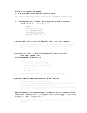
7a. List and explain four distance measures to compute the distance between a pair of points and find out the distance between two objects represented by attribute values (1,6,2,5,3) & (3,5,2,6,6) by using any 2 of the distance measures (08 Marks) Ans:
- EUCLIDEAN DISTANCE
- This metric is most commonly used to compute distances.
- The largest valued-attribute may dominate the distance.
- Requirement: The attributes should be properly scaled.
- This metric is more appropriate when the data is not standardized.
2) MANHATTAN DISTANCE
- In most cases, the result obtained by this measure is similar to those obtained by using the Euclidean distance.
- The largest valued attribute may dominate the distance.
3) CHEBYCHEV DISTANCE
- This metric is based on the maximum attribute difference.
4) CATEGORICAL DATA DISTANCE
- This metric may be used if many attributes have categorical values with only a small number of values (e. metric binary values).
where N=total number of categorical attributes
Solution: Given, (x 1 ,x 2 ,x 3 ,x 4 ,x 5 ) = (1, 6, 2, 5, 3) (y 1 ,y 2 ,y 3 ,y 4 ,y 5 ) = (3, 5, 2, 6, 6)
Euclidean Distance is
= 3.
Manhattan Distance is
D(x,y) = |x 1 -y 1 |+|x 2 -y 2 |+|x 3 -y 3 |+|x 4 -y 4 |+|x 5 -y 5 | =
Chebychev Distance is
D(x,y) = Max ( |x 1 -y 1 |,|x 2 -y 2 |,|x 3 -y 3 |,|x 4 -y 4 |,|x 5 -y 5 | ) = 3
Exam, answers
Course: Data Mining (IS ZC425)

- Discover more from: